
A discrete variable is a quantitative variable that can take only separate, countable values. Its possible values may be finite or countably infinite, but not every value between two points is permitted. Common examples include the number of students in a class, publications by a researcher and defects found in a product.

Introduction
Variables are characteristics that can differ between people, objects, events or observations. Correctly identifying a variable as discrete, continuous or categorical helps researchers decide how to collect the data, display its distribution, select a statistical method and interpret the results.
This article explains what a discrete variable is, how it differs from related variable types, how to identify difficult cases and how discrete variables are used in probability, data analysis and modern research.
Key Takeaways
- A discrete variable has a finite or countably infinite set of permissible values.
- Discrete variables are commonly obtained by counting, but they do not always consist only of whole numbers.
- A numerical category code is not automatically a discrete quantitative variable.
- The recorded format of a value does not necessarily determine the theoretical nature of the variable.
- Count outcomes often require methods such as Poisson or negative binomial regression rather than ordinary linear regression.
- Researchers should document the variable’s definition, unit, allowable values and measurement process.
What Is a Discrete Variable?
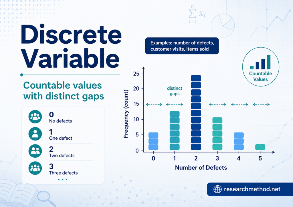
A discrete variable is a numerical variable whose possible values are distinct and countable. There are gaps between consecutive permissible values, meaning that some intermediate values cannot occur under the variable’s definition.
For example, the number of children in a household may be 0, 1, 2, 3 or another non-negative integer. It cannot be 2.4 children. The variable is therefore discrete.
A more formal definition is:
Discrete variable definition: A variable is discrete when its set of possible values is finite or countably infinite.
“Countably infinite” means that the possible values can be placed in a sequence, even when the sequence never ends. The number of emails received in a lifetime could theoretically take the values 0, 1, 2, 3 and so on. There is no fixed maximum, but the values remain countable.
Main characteristics of a discrete variable
A discrete variable generally has the following characteristics:
- It has distinct permissible values.
- Its possible values can be listed or placed in a sequence.
- There are gaps between permissible values.
- It is frequently produced by counting events, people or objects.
- Individual values can have non-zero probabilities in a probability model.
- It may have a finite or countably infinite range.
Examples of Discrete Variables
Common discrete variable examples include:
- Number of students enrolled in a course.
- Number of books borrowed from a library.
- Number of hospital visits during a year.
- Number of errors found in an examination paper.
- Number of research articles published by an academic.
- Number of customers arriving during an hour.
- Number of defective products in a batch.
- Number of correct answers on a 20-item test.
- Number of children in a household.
- Number of goals scored in a football match.
- Number of software crashes recorded during a week.
- Number of citations received by an article.
Examples from academic research
| Research field | Discrete variable | Possible values |
|---|---|---|
| Education | Number of absences during a semester | 0, 1, 2, 3, … |
| Healthcare | Number of hospital admissions | 0, 1, 2, 3, … |
| Psychology | Number of correctly recalled words | 0 to the total number presented |
| Business | Number of purchases made by a customer | 0, 1, 2, 3, … |
| Engineering | Number of component failures | 0, 1, 2, 3, … |
| Public health | Number of new cases in a region | 0, 1, 2, 3, … |
| Environmental research | Number of species observed at a site | 0, 1, 2, 3, … |
| Information technology | Number of login attempts | 1, 2, 3, … |
Discrete Variable vs. Continuous Variable
A discrete variable takes separate, countable values. A continuous variable can theoretically take any value within an interval, subject to the precision of the measuring process.
The simplest introductory rule is:
- Discrete variables are usually counted.
- Continuous variables are usually measured.
This rule is useful, but researchers should also examine the permitted value set and the way the variable is defined.
| Feature | Discrete variable | Continuous variable |
|---|---|---|
| Possible values | Separate and countable | Any value within an interval |
| Typical source | Counting | Measurement |
| Gaps between values | Present | Theoretically absent |
| Common values | Often integers | May include any decimal precision |
| Example | Number of patients | Patient body temperature |
| Probability function | Probability mass function | Probability density function |
| Common graph | Bar chart or dot plot | Histogram, density plot or box plot |
| Common models | Binomial, Poisson, negative binomial | Normal, gamma or continuous regression models |
Example: students and height
The number of students in a classroom is discrete because it can be 20 or 21 but not 20.4.
The height of each student is continuous because, in theory, height can take any value within a biologically possible interval. A recorded value such as 172.4 centimetres is only an approximation determined by the measuring instrument.
Do Discrete Variables Have to Be Whole Numbers?
No. A discrete variable does not have to contain only whole numbers. It must contain a countable set of separated permissible values.
Shoe size is a standard example. A sizing system may permit values such as 7, 7.5, 8 and 8.5 while excluding values such as 7.13 or 8.27. The variable is discrete because only specific steps are allowed.
Other possible decimal-valued discrete variables include:
- Prices restricted to fixed currency units.
- Scores awarded in half-point increments.
- Medication doses offered only in predetermined strengths.
- Ratings permitted in 0.5-point steps.
- Machine settings limited to fixed increments.
The presence of a decimal point therefore does not make a variable continuous. Researchers must ask whether every intermediate value is possible.
Discrete Variable vs. Categorical Variable
A discrete quantitative variable represents a numerical amount for which arithmetic operations are meaningful. A categorical variable represents group membership or a label.
This distinction is important because categorical variables are often stored using numbers.
For example:
0 = control group1 = treatment group
These numbers are category codes. Subtracting 0 from 1 does not represent a measured difference of one unit. The variable is binary and has discrete recorded values, but its substantive measurement level is categorical.
By contrast, the values 0, 1, 2 and 3 hospital visits represent actual counts. Differences and totals have meaningful numerical interpretations.
| Variable | Numerical appearance | Correct interpretation |
|---|---|---|
| Number of hospital visits | 0, 1, 2, 3, … | Discrete quantitative |
| Treatment group | 0 or 1 | Binary categorical |
| Satisfaction category | 1 to 5 | Ordinal categorical |
| Number of correct answers | 0 to 20 | Discrete quantitative |
| Postal code | Numeric digits | Nominal identifier |
| Temperature | Numeric measurement | Continuous quantitative |
Are binary variables discrete?
A binary variable has two possible values, so its value set is discrete. However, researchers normally classify it more specifically according to its meaning.
A yes/no response, disease status or treatment-group indicator is usually analysed as a binary categorical variable. A Bernoulli random variable is the corresponding probability concept when the two outcomes are represented numerically as 0 and 1.
How to Identify a Discrete Variable
Use the following five-step process.
Step 1: Define what the variable represents
Write an operational definition. Do not classify a variable from its name alone.
For example, “age” may mean exact elapsed time since birth or completed years recorded on a questionnaire. These definitions produce different recorded variables.
Step 2: Identify all permissible values
Ask which values could occur under the definition.
If the variable is “number of children,” the permissible values are 0, 1, 2 and other whole-number counts. If the variable is “body mass,” any value within a plausible interval is theoretically possible.
Step 3: Look for impossible intermediate values
Ask whether another permissible value exists between two neighbouring values.
There is no permitted value between two and three children. By contrast, many possible body masses lie between 70 and 71 kilograms.
Step 4: Separate the construct from its recorded precision
A continuous construct can be recorded in discrete increments. A thermometer may display temperature to one decimal place, but rounding does not necessarily change temperature into a naturally discrete phenomenon.
Step 5: Check how the variable will be analysed
Determine whether the variable represents:
- A count.
- A binary outcome.
- An ordered category.
- An unordered category.
- A measurement rounded to fixed precision.
- A rate or proportion.
- A grouped version of a continuous variable.
The appropriate analysis depends on this substantive meaning rather than the spreadsheet format alone.
Ambiguous Examples
Is age discrete or continuous?
Exact age is continuous because elapsed time can theoretically be measured with increasingly fine precision. Age in completed years is a discrete recorded variable because only whole-year values are retained.
Researchers should report which definition they used. Treating age as continuous in a regression model may be reasonable when the scale has many values and the relationship is appropriately modelled, but the choice should be justified.
Is money discrete or continuous?
Money is technically discrete when transactions are restricted to the smallest currency unit, such as cents or pence. In many economic models, however, monetary values are treated as approximately continuous because the unit is small relative to the values being studied.
The research context, currency rules and modelling purpose should determine the treatment.
Is GPA discrete or continuous?
A GPA is discrete when an institution permits only a fixed set of reported values or calculates it from a finite combination of grades and credit weights. It is often treated as approximately continuous in applied analysis when it has many possible values.
Researchers should not call every GPA scale continuous without checking how the institution calculates and records it.
Are test scores discrete?
A raw score based on the number of correct answers is discrete. On a 20-item test, the score may take only the values 0 through 20.
A transformed or standardised score may have many decimal values, but it can still originate from a discrete raw score. The level at which the analysis is performed should be stated.
Are Likert-scale responses discrete?
A single Likert item, such as a response from “strongly disagree” to “strongly agree,” is an ordinal categorical variable with a finite set of possible responses.
A total score created by adding several items is a discrete numerical score. Researchers sometimes analyse a sufficiently broad multi-item scale as approximately continuous, but this is an analytical decision rather than proof that the underlying responses are continuous.
Is time discrete or continuous?
Time is theoretically continuous in many scientific models. It becomes a discrete recorded variable when observations are restricted to fixed points or units, such as completed days, monthly survey waves or one-second timestamps.
The underlying phenomenon and the observation schedule should not be confused.
Discrete Variable and Discrete Random Variable
A variable in a dataset is a characteristic recorded for each observation. A random variable is a function that assigns a numerical value to each possible outcome of a random process.
A discrete random variable has a finite or countably infinite set of possible values.
For example, let (X) represent the number of heads obtained in three coin tosses. The possible values are:
[
X = 0, 1, 2, 3
]
The variable is discrete because only four values are possible.
Probability mass function
A probability mass function, or PMF, assigns a probability to each possible value of a discrete random variable:
[
p(x)=P(X=x)
]
A valid PMF satisfies two conditions:
[
0 \leq p(x) \leq 1
]
and
[
\sum_x p(x)=1
]
Unlike a continuous random variable, a discrete random variable can assign positive probability to an exact individual value.
Expected value
The expected value is the probability-weighted long-run mean:
[
E(X)=\sum_x xP(X=x)
]
The expected value does not have to be one of the variable’s possible outcomes. For a fair six-sided die, the expected value is 3.5, even though a single roll can never produce 3.5.
Variance
The variance describes the spread of a discrete random variable around its expected value:
[
Var(X)=\sum_x [x-E(X)]^2P(X=x)
]
An equivalent formula is:
[
Var(X)=E(X^2)-[E(X)]^2
]
The standard deviation is the square root of the variance.
Common Discrete Probability Distributions
| Distribution | Typical use | Example |
|---|---|---|
| Bernoulli | One trial with two outcomes | Whether a participant completes a programme |
| Binomial | Number of successes in a fixed number of independent trials | Correct answers out of 20 questions |
| Poisson | Number of events in a defined exposure period or area | Calls received per hour |
| Geometric | Number of trials until the first success | Attempts required before successful login |
| Negative binomial | Overdispersed counts or trials until a specified number of successes | Repeated event counts with greater variability than a Poisson model |
| Hypergeometric | Successes sampled without replacement from a finite population | Defective items in a sample from a batch |
A distribution should not be chosen only because a variable is discrete. Its assumptions must match the data-generating process.
Collecting and Recording Discrete Variables
A strong research protocol should specify:
- The variable name.
- Its conceptual and operational definitions.
- The unit of observation.
- Its allowable values.
- The reference or exposure period.
- Whether zero is possible.
- Whether an upper limit exists.
- How missing and impossible values will be coded.
- Whether repeated events can occur.
- Whether the value is a count, category, proportion or rate.
For example, “number of clinic visits” is incomplete unless the protocol also specifies the period, eligible clinic types, whether cancelled visits count and how records from multiple systems will be reconciled.
Count versus rate
A count records the number of events. A rate relates that count to exposure, time or population size.
Ten accidents in a small factory and ten accidents in a large factory do not necessarily represent the same level of risk. The analysis may need an exposure variable, such as employee-hours, and a count model with an offset.
How to Present Discrete Data
Frequency table
A frequency table reports each value and the number or percentage of observations with that value. It is especially useful when the number of distinct values is small.
Bar chart
A bar chart displays separated bars for individual values or categories. The gaps visually communicate that intermediate values are not observed or permitted.
Dot plot
A dot plot can show the distribution of a small or moderately sized dataset without hiding individual observations.
Histogram
A histogram may be useful when a discrete variable has many ordered values, but researchers should select bin widths carefully. For small integer counts, a bar chart or count plot usually communicates the discrete structure more clearly.
Probability mass plot
For a theoretical discrete random variable, a PMF plot shows each possible value and its associated probability.
Statistical Analysis of Discrete Variables
The appropriate method depends on whether the variable is a count, binary outcome, ordered category or another form of discrete data.
| Research situation | Common analytical approach |
|---|---|
| Describe a count variable | Frequencies, percentages, mean, median, variance, range |
| Compare a binary outcome between groups | Contingency table, risk difference, risk ratio, odds ratio, logistic regression |
| Analyse an unordered categorical outcome | Chi-square procedures or multinomial logistic regression |
| Analyse an ordered categorical outcome | Ordinal summaries or ordinal logistic regression |
| Model an event count | Poisson or negative binomial regression |
| Model successes from a fixed number of trials | Binomial model |
| Analyse counts with many zeros | Zero-inflated or hurdle model when substantively and statistically justified |
| Analyse repeated discrete outcomes | Generalised estimating equations or mixed-effects generalised models |
| Analyse event rates | Poisson or related count model with an exposure offset |
Can the mean be calculated?
Yes, the mean can be meaningful for a discrete quantitative variable. A sample might average 2.4 hospital visits per patient even though no individual patient made exactly 2.4 visits.
The mean should not be calculated merely because categories have been assigned numbers. For example, the mean of arbitrary postal-code numbers has no substantive interpretation.
Why ordinary linear regression may be inappropriate
Linear regression can predict impossible negative counts, assume constant variance and poorly represent strongly skewed or zero-heavy outcomes.
Poisson regression is a standard starting point for event counts. However, the Poisson model assumes a specific mean–variance relationship. When the observed variance is substantially greater than expected, a negative binomial model or another extension may be more appropriate.
Researchers should examine the distribution, exposure period, excess zeros, clustering and model diagnostics instead of selecting a method solely from the word “discrete.”
Advantages of Discrete Variables
Discrete variables can offer several practical advantages:
- Values are often straightforward to define and verify.
- Exact event counts can be easy to interpret.
- Impossible values can be identified through validation rules.
- Frequencies and probabilities are easy to communicate.
- Many established probability distributions and specialised models are available.
- Counts often correspond directly to operational decisions, such as staffing, inventory or service demand.
Limitations and Practical Challenges
Discrete data can also create difficulties:
- Small value sets produce many tied observations.
- Floor and ceiling effects may limit variability.
- Counts may be highly skewed.
- Many observations may equal zero.
- Different participants may have unequal exposure periods.
- Values may be undercounted because of incomplete records.
- Converting continuous data into categories can remove information.
- A high-count variable may appear continuous even though it remains theoretically discrete.
- Standard software defaults may not select the correct measurement level or model.
Common Mistakes
Assuming that every numerical variable is quantitative
Numbers may be identifiers or category labels. Researchers must interpret what the values mean.
Assuming that decimals always indicate continuity
Fixed decimal steps can form a discrete set.
Assuming that all discrete variables are finite
A discrete variable may have a countably infinite set of possible values.
Classifying a variable from observed values only
A sample may contain only 10, 20 and 30, while the variable itself permits every real value between them. Classification should reflect the possible value set, not only the values that happened to be observed.
Confusing rounding with natural discreteness
A continuous measurement recorded to two decimal places remains an approximation of a continuous construct.
Treating a single Likert item as an interval-scale measurement without justification
The numerical labels indicate ordered response categories. Equal numerical spacing does not automatically establish equal psychological distance.
Ignoring the observation window
“Number of events” must normally be linked to a defined period, location, population or other exposure.
Using Poisson regression without checking dispersion
Count data can show overdispersion, underdispersion or excess zeros. Model assumptions and diagnostics remain essential.
Discrete Variables in Modern Research
Discrete variables appear throughout contemporary research:
- Electronic health records contain counts of visits, diagnoses and prescriptions.
- Learning-management systems record submissions, logins and completed activities.
- Digital platforms track clicks, comments, purchases and sessions.
- Environmental systems record detected species and threshold exceedances.
- Genomic studies analyse sequencing read counts.
- Cybersecurity research examines attacks, login failures and malware detections.
- Manufacturing systems count defects, interruptions and rejected units.
Modern datasets often combine discrete counts, categorical labels, continuous sensor measurements, text, images and timestamps. Researchers therefore need a documented data dictionary rather than relying on a software package to infer each variable’s meaning.
Digital Tools, Software and Artificial Intelligence
Statistical software
SPSS, R, Python, Stata, SAS and spreadsheet programs can store and analyse discrete variables. However, the storage type and measurement level are not identical concepts.
An integer column may contain:
- A genuine count.
- A binary indicator.
- An ordinal category.
- A nominal code.
- A continuous measurement rounded to whole units.
Researchers should manually verify variable definitions and software settings. Automatic classification based on the number of unique values can be useful, but it can also misclassify variables.
R and Python
R supports binomial and Poisson generalised linear models through standard modelling functions, with additional packages available for negative binomial, mixed and zero-inflated models.
Python libraries support integer and categorical data types, probability distributions, count visualisations and generalised linear models. The researcher must still select a model that matches the study design and assumptions.
Using generative AI
Generative AI can assist with:
- Suggesting an initial variable classification.
- Creating data-dictionary templates.
- Explaining statistical output.
- Producing draft R or Python code.
- Identifying impossible values.
- Generating practice examples.
AI output should not be treated as a final methodological decision. AI systems may confuse category codes with quantities, overlook the study’s operational definition or recommend a statistical test without checking assumptions.
Researchers should remove or protect confidential data, follow institutional policies, verify generated code and retain human responsibility for the final analysis. UNESCO’s guidance on generative AI in education and research emphasises privacy, transparency, human oversight and a human-centred approach.
How to Report a Discrete Variable in a Research Paper
A methods section should explain:
- What the variable represents.
- How it was measured or counted.
- Its possible or observed range.
- The reference period.
- Any transformations or category groupings.
- The descriptive summaries used.
- The statistical model and why it was appropriate.
- How missing, impossible or extreme values were handled.
Reporting example
The outcome was the number of emergency-department visits recorded for each participant during the 12-month follow-up period. It was treated as a non-negative count variable. Because the variance exceeded the mean, negative binomial regression was used instead of a Poisson model. Follow-up time was included as an exposure offset.
This description is more informative than simply stating that the outcome was “discrete.”
Conclusion
A discrete variable takes separate, countable values and contains gaps between permissible values. Although discrete variables commonly represent whole-number counts, they may also use fixed decimal increments. Correct classification requires examining the variable’s meaning, permissible values, measurement process and planned analysis—not merely its appearance in a spreadsheet.
Distinguishing counts from categories and rounded measurements helps researchers choose appropriate summaries, graphs, probability distributions and statistical models.
References
Australian Bureau of Statistics. (n.d.). Variables. Retrieved June 22, 2026.
- Heckert, N. A., Filliben, J. J., Croarkin, C. M., Hembree, B., Guthrie, W. F., Tobias, P., & Prinz, J. (2002). NIST/SEMATECH e-handbook of statistical methods (NIST Handbook 151). National Institute of Standards and Technology.
- IBM. (n.d.). Variable measurement level: IBM SPSS Statistics. Retrieved June 22, 2026.
- Illowsky, B., & Dean, S. (2023). Introductory statistics 2e. OpenStax.
- Miao, F., & Holmes, W. (2023). Guidance for generative AI in education and research. UNESCO.
- Monash University. (n.d.). Discrete random variables. Retrieved June 22, 2026.
- Pennsylvania State University. (n.d.). Analysis of discrete data: STAT 504. Retrieved June 22, 2026.


